This article was originally published on LessWrong.

Motivation

Dimensionality reduction is vital to the analysis of high dimensional data, i.e. data with many features. It allows for better understanding of the data, so that one can formulate useful analyses. Dimensionality reduction that produces a set of points in a vector space of dimension n, where n s much smaller than the number of features N in the data set. If the number n is 1, 2, or 3, it is possible to visualize the data and obtain insights. If n is larger, then it is more difficult. One interesting situation, though, is where the data concentrates around a non-linear surface whose dimension is 1, 2, or 3, but can only be embedded in a dimension higher than 3. We will discuss such examples in this post. If we want to take advantage of the fact that the dimension of the surface is lower than the dimension of the embedding space, we need new tools for representing the surface. In this post, we will talk about the representation techniques, and in future posts we’ll discuss how they can be used.

Nonlinear Surfaces

Non-linear surfaces can sometimes be represented as the vanishing sets of polynomials or sets of polynomials. For example, a torus can be described as the subset of R4 consisting of the points satisfying the two equations x2+y2=1 and z2+w2=1. One problem with this mode of representation is that it is often difficult to find the right algebraic equations for the surface. Even when one can, it is difficult to work with the algebraic description. For example, it can be very difficult to sample from the surface, and it is difficult to describe distributions on it. One way of getting around this is by introducing intrinsic coordinates, as one does when one introduces the single angular coordinate θ on the circle or intrinsic coordinates θ1 and θ2 for the torus. Although this can be done for a number of surfaces, for example by introducing spherical harmonics for spheres, it typically requires very detailed analysis, and there are many situations where there are no particularly natural choices for intrinsic coordinates. Another way of describing a surface is by triangulation. This means describing the surface as a collection of simplices, i.e. points, intervals, triangles, tetrahedra, and higher dimensional analogues.

Figure 1: Triangulations of a sphere and of a torus

This kind of representation of a surface can be very useful, due to the fact that it is an intrinsic description of the surface. This means that it represents the points on the surface without reference to any particular vector embedding, so that the dimension is reduced to the actual dimension of the surface, rather than to the dimension of a vector embedding. We'll describe two examples of data sets where the data is concentrated around a surface or a curve, which is of lower dimension than the natural vector embedding of the data.

The Loop

Our first example is the Jena Climate Data Set. It is a study of various climatic quantities constructed by the Max Planck institute, collected from their weather station in Jena. It is equipped with 14 total features, but to remove redundancy (say of temperature in Celsius and Kelvin, for example) we selected four features, namely temperature in Celsius, relative humidity, maximum vapor pressure, and actual vapor pressure. One available feature is time, at a fairly fine scale, and we have removed it. The data was collected from January of 2009 to December of 2016. The question is whether we can recover the any aspect of the time variable from this data. We performed Principal Component Analysis (PCA) , and obtained the following scatter plot.

This analysis is available as a colab notebook.

It is apparent that there is some organization of the data around a loop. A reasonable hypothesis is that data for the first week of November in all years will be roughly similar, so we will not be able to tell what year, only approximately the day or week during any of the years. The loopy structure also suggests the possibility of a single angular coordinate θ which could be generated for the data, so that instead of obtaining a two-dimensional dimensionality reduction, we have a one-dimensional one. We pay the price of having to restrict to the range from 0 to 2π, or recognizing that the parameter should be viewed as periodic with period 2π.

The Klein bottle

We'll now look at a more complicated example. It comes from a paper by Anne Pedersen et al concerning the statistical structure of natural images. In this case, the data set they constructed (which we'll call the Mumford data) consists of roughly 8 million 3×3image patches, collected from a database of roughly 5000 gray scale images taken around Groningen in the Netherlands. The images were obtained in a paper by van Hateren and van der Schaaf, and the patches were in Pedersen et al. The image patches are represented as 9-dimensional vectors, with one gray scale value at each pixel in a 3×3square array in the image. In Figure 3 below, you see an array of 25 such patches from Pedersen et al

In examining data sets of image patches, it is important to filter out patches which are essentially constant, since such patches will likely dominate the statistics, washing out the behavior of highly non-constant, or high variance, patches. Pedersen et al constructs a data set which filters out low variance patches, and therefore consists of high variance patches. In Carlsson et al, an analysis was performed which showed that the densest part of the data set from Pedersen et al is actually concentrated around a subset which is parametrized as a Klein bottle (see Figure 4 below). A Klein bottle is a mathematical object called a manifold which is a high dimensional analogue of a surface. Manifolds include surfaces of all dimensions, and the Klein bottle is a 2-dimensional surface. In a way similar to the way the circle is coordinatized by a single parameter θ, the Klein bottle can be parametrized by two parameters θ1 and θ2 with the understanding that like the parameter θ for the circle, and are restricted to finite ranges, or obey a somewhat complicated periodicity.

We have not described how it is that Carlsson et al were able to determine that the data was concentrated around a Klein bottle. For surfaces of all dimensions, there are characteristic numbers called Betti numbers which are attached to them. See this book for an introduction. For every non-negative integer i, there is a Betti number (a non-negative integer) βi which is attached to every manifold. The integer β0 is a count of the number of connected components, β1 is a count of the number of loops which are independent in an appropriate sense, and the higher Betti numbers are usually thought of as counting the number of "k-dimensional holes", suitably defined, in a surface or manifold. Additionally, it turns out that there is a complete classification of 2-dimensional surfaces, described in detail in Gallier and Xu, A Guide to the Classification Theorem for Compact Surfaces, or in a novel proof from a different point of view. They are classified by a pair (g,i), where g is a non-negative integer called the genus, and where i=±1. The parameter i reflects orientability / non-orientability. Orientability is a property of surfaces which determines whether the surface is “one-sided”, like the Klein bottle, or two-sided, like the sphere or the torus. The Klein bottle corresponds to the pair (1,−1), and Carlsson et al were able to establish that the Betti numbers for the Mumford data set corresponded to the pair (1, -1).

An important fact about the Klein bottle K is that although it is defined as a manifold, it cannot be realized as a surface in 3-dimensional space, but can be realized as a 2-dimensional surface in 4-dimensional space, R4. The reason this fact is important is that unlike the circle, which can be visualized, it is not possible to see K, due to the fact that the space we live in is 3-dimensional. For this reason, the idea of applying a 2 or 3 dimensional PCA to this data will not exhibit the result accurately. It can be defined by two equations in four variables, but those equations are hard to discover. For example, while there is a single standard embedding of the circle in R2, there is not a single “most natural” embedding of K in R4. This means that it is desirable to find an intrinsic way to represent K.

Other Examples

There are a number of examples where the topology of a data set is of importance. One situation is the study of conformation spaces of molecules. Jose Perea and collaborators have done a great deal of interesting work in this direction. What the authors find is a description of the spaces of conformations of pentane (it is a Moebius band) and cyclooctane (a complicated space which is a union of a Klein bottle and a sphere, glued together along two circles). Also, E. Moser et al have studied activation spaces of neurons involved in mapping surrounding regions and found that in the simplest analysis their result is a torus.

Topology

The pattern that we have seen in these two examples is that we have data that is presented to us as high-dimensional (4 dimensions in case of the Jena set and 9 dimensions in the case of the Mumford data), but nevertheless could be represented as a manifold of lower dimension. In the first example, the results are concentrated around a loop (which is a one-dimensional object) embedded in 2-dimensional space. As we saw, it is concentrated around an ellipse, which can be defined by a simple degree two equation of the form x2a2+y2b2=1. In the second case, the surface K is intrinsically 2-dimensional, and cannot be embedded as a surface in three dimensions but requires four. As an alternative to searching for equations defining the manifolds, we want to introduce a method for representing the surface which is intrinsic, i.e. depends only on the points of the data set and the distances between them, and not on a particular vector embedding.

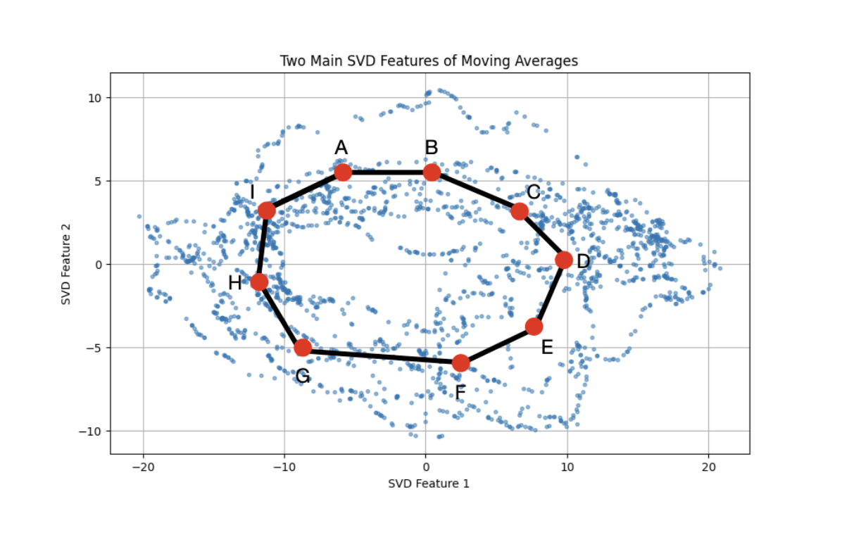
To illustrate the process, let's consider the Jena data set again. Earlier we approximated it by the zero set of an algebraic equation, the equation for an ellipse. In Figure 5 below, we approximate it instead by a graph on 9 vertices labelled by A,B,C,D,E,F,G,H, and I.

The graph is defined by the requirements that the pairs

{{A,B},{B,C},{C,D},{D,E},{E,F},{F,G},{G,H},{H,I},and{A,I}

comprise all the pairs of vertices connected by edges. The graph structure determines the space in the following sense. It is possible to place all the vertices of the graph in the plane or in space and connect all the pairs of points listed above as edges, and to do so in such a way that none of the edges intersect any of the other edges. Any two choices of such "vertex embeddings" give spaces that are homeomorphic in the sense that there is a continuous mapping f from one to the other so that the points of the two embeddings are in one to one correspondence via f. The process of building a graphs associated to spaces is a one-dimensional example of a process called triangulation. This terminology comes from the fact that one can apply the same idea to higher dimensional spaces. For instance, in Figure 1 above, the sphere and the torus are represented as objects called simplicial complexes, which are higher dimensional analogues of graphs. In 2-dimensional simplicial complexes, rather than only having edges represented by pairs, one also has “2-simplices” (which are triangles) represented by triples of vertices. In higher dimensions, one has objects called n-simplices, which are represented by n+1-tuples of vertices. The definition of simplicial complexes is purely combinatorial, in that they can be specified by purely combinatorial descriptions consisting of a family of subsets of the vertex set. For example, the boundary of a tetrahedron

is described by the family of sets

{0},{1},{2}

{0,1},{0,2},{0,3},{1,2},{1,3},{2,3}

{0,1,2},{0,1,3}{1,2,3},{1,2,3}

If we added the total set {0,1,2,3}, this would correspond to the the solid tetrahedron. The Klein bottle can be triangulated, and there is a relatively simple triangulation with 18 triangles. Unfortunately, it is hard to visualize. There is a simple way of understanding the Klein bottle via identification spaces. The simplest example of an identification space is a Moebius band, where one cuts a strip of paper and then glues the two ends together “with a twist”, i.e. so that the bottom of the left hand edge is identified with the top of the right hand edge.

There is a similar construction for the Klein bottle.

Figure 8: Identification space description of Klein bottle

Here we take a piece of paper and identify the red edges on the top and bottom, without a twist, and the blue edges on the left and right with a twist. You can try to do this with a piece of paper, and you will invariably be forced to tear the paper. This fact reflects the fact that the Klein bottle cannot be viewed as a manifold in R4.

To conclude, here is an image which indicates the relationship between the Klein bottle and the Mumford data set of image patches.

Figure 9: Image patches laid out on Klein bottle

Notice that the left and right edges are identified with a twist and the upper and lower edges do not have a twist. The finding here is that the image patches that occur most frequently include edges between black and white regions with a linear boundary, as well as black (or white) lines on a white (or black) background. Jose Perea has used these findings for studying textures, and in joint work with Ephy Love, Ben Filippenko, and Vasileos Maroulas we have producing neural networks for images that generalize better than standard methods.

Applications to Data Science

There are some questions that deserve answering.

How do we arrive at topological models?

One general method is via the nerve construction, which we discussed in our earlier post It is the basis for the Mapper method and its variants. If one has an a priori understanding of the underlying space via Betti numbers or other approaches, once can build coverings designed to take that understanding into account.

How do we use the topological model for data science tasks such as feature generation and engineering?

There is an important area of applied mathematics called graph signal processing, which finds eigenfunction decompositions of the space of functions on a graph. This field includes the usual discrete Fourier transform, which applies to cyclic or toroidal graphs, but which has extensions to all graphs. Similarly, there is a very nice construction for functions on the Klein bottle. These techniques produce functions on the vertices of a graph or simplicial complex. If the graph is the nerve of a covering of a data set, one can use interpolation techniques to construct features on the data set itself.

Can topological modeling be used to obtain equations describing a data set?

Although we have argued that there are some difficulties with algebraic representations of data sets as zero sets of equations or systems of equations, it is sometimes desirable or necessary to find such representations. In that case, it is critical to determine what is being represented by the equations. For example, given that the underlying space is a Klein bottle, there are many different embeddings for different tasks one might use, which can be understood with algebra. Without the understanding that the data set is concentrated around a particular manifold, one cannot get started in designing useful embeddings.

We’ll flesh these points out in future posts.

From Loops to Klein Bottles: Uncovering Hidden Topology in High Dimensional Data

How to Use BluelightAI Cobalt with Tabular Data