By Zahra Rostami, David Fooshee, Gunnar Carlsson, and Shankar Subramaniam, in collaboration with The Department of Computer Science and Engineering at University of California, San Diego, BluelightAI, and The Department of Mathematics at Stanford University
This paper was originally published in the IEEE Open Journal of Engineering in Medicine and Biology.
Impact Statement:
High dimensional data is difficult to visualize or analyze. Reducing the dimension of data while preserving its veracity has become a key challenge for data science. A key tenet of data is its shape that can be topologically defined. In this study, we use the shape or topology of data to infer features that potentially carry valuable information. We use BC data as an example owing to its importance and complexity. The heterogeneity of BC data makes interpretation and prognosis difficult. We show that topological analysis of BC data and its graphical representation provide a natural subtyping in addition to parsing the associated features. Interestingly, the topological analysis points to a novel HER-2 positive luminal subtype, suggesting alternate therapeutic interventions.
Abstract:
Objective: High-throughput biological data, with its vast complexity and higher dimensions, continues to require innovative analytic methodologies for meaningful exploration. Most methods for reducing data dimensions overlook the shape and topology of data, even though these are vital components of the data structure and complexity. This study leverages topological data analysis (TDA) and shows, using breast cancer (BC) gene expression data as an illustrative example, the power of including the shape of data.
Results: In addition to delineating the known subtypes of BC, TDA identifies a new subtype within luminal B cancer along with the features that define the subtype. The final outcome is shown via three-dimensional (3D) scatter plots which demonstrate how the underlying patterns that we identified through TDA map to 3D space.
Conclusions: The new subtype, obtained unsupervised and validated by prior knowledge, demonstrates the power of embedding the topology and shape of data in the analyses.

Introduction
High-throughput biological data contains invaluable information, but is typically large-dimensional, noisy, and complex. Additionally, biological systems inherently exhibit high variability, and the changes in the notion of distance or similarity in biological data are less definable rigidly. Therefore, extracting useful information from these datasets is a challenge, and the more distance-rigid methods like Principal Component Analysis (PCA) often fall short. TDA seeks to address this challenge. A particular methodology within TDA is graph modeling, which represents the shape of data by a graph. Methods like Mapper and the Insights construct graphs where nodes correspond to subsets of data, connected based on similarity criteria, offering discretized analogues of Reeb graph constructions The graphs can provide an understanding of the overall organization of the data by leveraging its shape. When there are a large number of features, it is useful to create graph models of the set of features, e.g., of the columns of a gene expression data matrix if the features (genes) are represented in columns.
TDA represents data in a flexible, dimensionless space, and analyzes both feature and sample structures simultaneously enabling a more integrated analysis of how and at what level features contribute to each part of the data. Such analyses are crucial in feature identification and engineering. We provide here the details and capabilities of such modeling. First, a predefined group of data points (rows in a data matrix) induces a function (displayed as a coloring) on the nodes of the graph model. For example, in a gene expression data across patients with a given disease with multiple subtypes, each subtype can be assigned a color. In this example, each node of the graph model represents a group of samples (rows) sharing similar gene expression profiles. The nodes can then be colored to indicate the subtype(s) of the samples they encompass. Second, a region of the graph model can be selected, and it determines a collection of data points. This, in the previous example, results in selection of the patient samples that belong to the groups associated with the nodes in the selected graph region. Third, each feature (or collection of features) can be viewed as a function on the samples. Thereby, the graph model of the data points, where nodes correspond to samples, may be colored by given feature(s). This can be done by first combining the features (if more than one feature is selected) using an aggregation function, such as mean or median, to get a single value for each sample. Then the aggregated values are averaged over the samples corresponding to node u, and the final numerical value of u is assigned a color in a systematic way. Similarly, the data points can be assigned to a function on the nodes of a graph model of the feature space by first aggregating over the selected data points and then averaging the results over the features corresponding to node v. In particular, if we also have a graph model of the data points (rows), we obtain a method for coloring the nodes of the graph model of the feature space (columns) based on nodes or sets of nodes of the model of the data points. These methods are helpful in analyzing data sets.
In this paper, we use these methods to uncover structure in gene expression data of BC patients. BC is a heterogeneous disease and based on hormone receptors (HR) and human epidermal growth factor receptor 2 (HER2), it is characterized by four main subtypes: luminal A (HR+, HER2-), luminal B (HR+, HER2+), HER2-enriched (HR-, HER2+), and TNBC (HR-, HER2-). Each subtype exhibits distinct clinical characteristics with specific therapeutic implications, making accurate subtype classification pivotal for tailoring treatment strategies, enhancing patient outcomes, and ideally achieving personalized treatment regimens.
Previous work by Nicolau et al. applied TDA techniques to study the sample (row) space of BC gene expression data, identifying a subgroup of cancer. Our current study introduces a methodological advancement by incorporating a graph model of the feature (column) space in addition to the sample space. This dual-space approach is essential, as it becomes a tool for feature selection. Here we show how the interplay between the model of the rows (samples) and columns (genes), described above, in our data matrix not only results in a robust delineation of the BC subtypes but also uncovers finer granularity within the subtypes, notably in luminal B, by distinguishing between HER2-low and HER2-high BC samples. Moreover, we demonstrate how this approach can help narrow down the features and identify key genes that play a distinctive role for each subtype.
We use the discoveries from our topological method to construct straightforward 3D scatterplots, where the axes are expression levels of individual genes that we identified. These scatterplots represent the structure of the data set well, and clearly illustrate the main finding, which is that there are groups of luminal B tumors for which the HER2 levels are lower than expected for HER2+ tumors. We emphasize that although we use TDA to find the structure, the final output is a scatterplot of the data using which other investigators can compare their results.
Results and Discussion
We used TDA as an exploratory tool in the analysis (see Materials and Methods for the details), and in this section, we present the steps we took to find the structure of the data. The result, which is the quantitative 3D scatter plot models, discussed in Section II-F, enables evaluating expression levels of the genes and identifying the subtype association of each sample. Towards this, we first identified shape characteristics of our data using TDA and generated our sample and feature networks (explained below). We then explored the introduction of additional partitions driven by the data itself and here we demonstrate how it resulted in separation of the BC subtypes. Finally, we show how the underlying patterns observed in the graph model is reflected in 3D space.
A. BC Sample Network
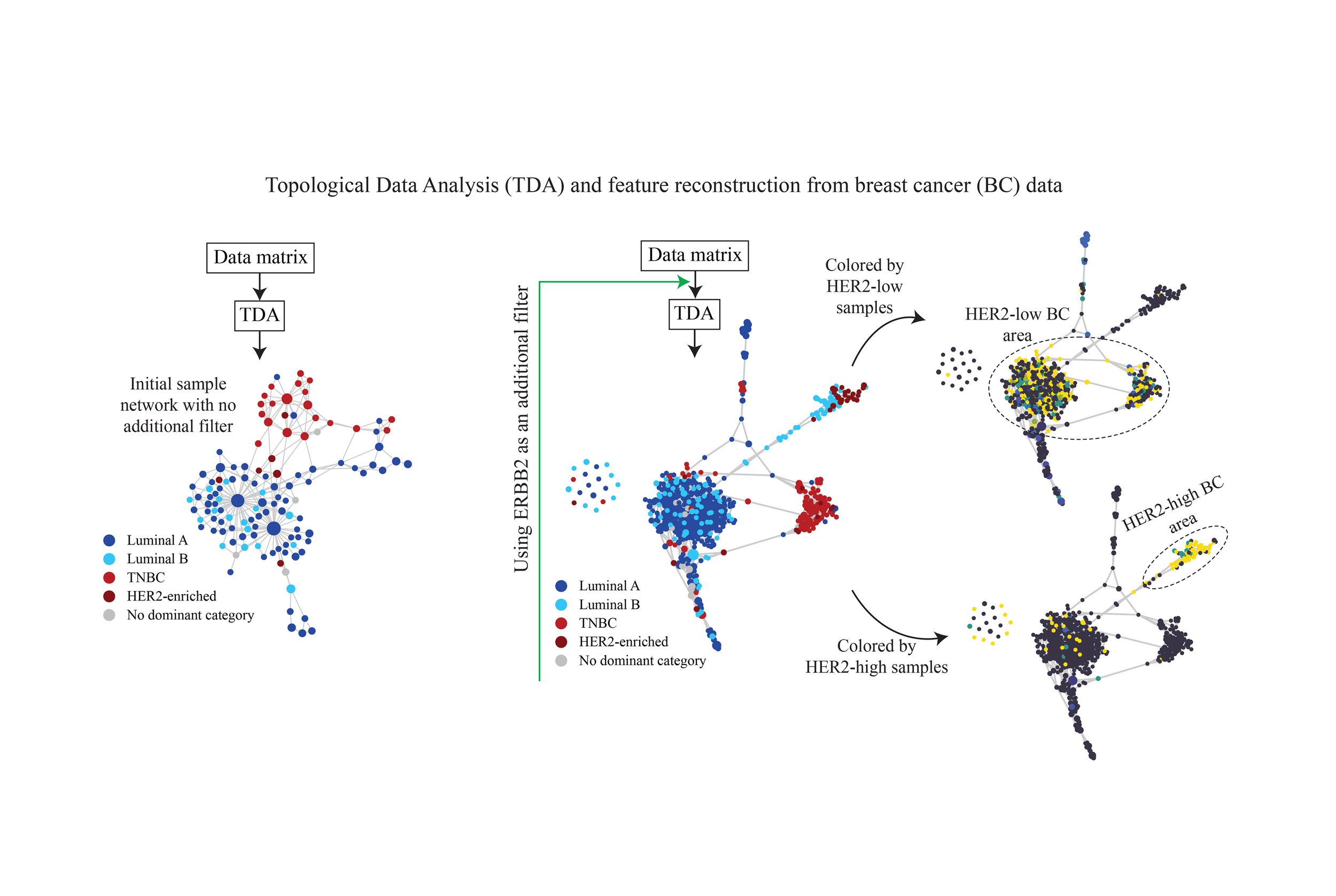
We followed the steps described in the Materials and Methods section and developed a topology-based approach using the BC gene expression data derived from TCGA (https://www.cancer.gov/tcga) to infer a sample-sample similarity network. In the resulting network, cancer samples (nodes) are connected to each other if they are similar in terms of their gene expression profile. Samples that exhibit extremely high level of similarity are grouped into a single node. Figure 1(a) shows the output where each node is a cluster of samples, and its color encodes the dominant BC subtype in that cluster. Dark blue, light blue, red, and brown nodes indicate the dominant subtype is luminal A, luminal B, TNBC, and HER2-enriched, respectively. We used Euclidian distance for the metric and L1 eccentricity for the filter to generate this network. L1 eccentricity, highlights outliers or extreme data points within the dataset. It achieves this by segregating points that, on average, exhibit significant distance from all other points, effectively partitioning them into distinct bins before graph construction. Consequently, it tends to isolate extreme data points, while central data points are clustered together, forming denser hubs.
In Figure 1(a) we see that TNBC is readily distinguishable from the others, forming a distinct cluster. In contrast, luminal A and luminal B subtypes exhibit a distributed pattern, appearing throughout the remaining areas of the network where TNBC is not dominantly present. HER2-enriched BC, characterized by its limited sample count, maintains its own nodes, and primarily resides in the vicinity of the TNBC area.
B. BC Feature Network
Similarly, we generated a feature network where each node is a cluster of features (genes). This network was created by applying the same TDA method on the transposed data matrix where genes become the rows and samples are represented in columns. For this network, correlation distance and L1 eccentricity was used as the metric and the filter, respectively. Figure 1(b) represents this network colored by samples with HER2 Immunohistochemistry (IHC) 3+ score (HER2-high). IHC test, a commonly used method to measure the HER2 receptor protein on the surface of the cell, gives a score of 0 to 1+, 2+, and 3+. According to traditional approaches, a score of 3+ is called HER2-positive and below this threshold, the cancer cells are considered HER2-negative as they do not benefit from conventional HER2-targeted treatments.
We used z-score normalized values for the colorings of all our feature networks to be able to compare the values of distinctive features. The highlighted bright yellow area in Figure 1(b), for example, indicates that HER2-high samples exhibit notably elevated values for the features in this specific region, as compared to the dataset as a whole. In this region, there are two nodes with the largest mean z-score values. Figure 1(c) shows these nodes along with their corresponding genes (ERBB2, PSMD3, STARD3, GRB7, PGAP3, MIEN1) indicating a strong correlation with HER2-high samples, which is supported by prior experimental studies. ERBB2, also known as HER2, is a critical biomarker in BC research. It encodes a protein involved in cell growth and proliferation and is known for its role in the development and progression of certain BC subtypes. PSMD3 is reported to control BC through stabilizing HER2 from degradation. STARD3 has shown a significant genetic and biological association with HER2 and is considered a potential biomarker for HER2+ BC. GRB7 and PGAP3 are known to be strongly co-expressed with HER2, and together, they have been found to be reliable predictors of HER2 status. MIEN1, located very close to ERBB2 gene on the long arm of chromosome 17, promotes cell migration and motility. Due to its proximity to ERBB2, it is usually overexpressed alongside ERBB2 in many BC cells.
C. Partitioning BC Sample Network Using Additional Filters
Our method enables emphasizing distinct aspects of the data by additional data partitions. We used ERBB2, one of the genes we identified in the previous step, to construct our additional data partition. The overexpression or amplification of ERBB2 is associated with aggressive tumor behavior, making it a pivotal target for therapeutic intervention and a key focus in our study. Using ERBB2 as the additional partition resulted in the network shown in Figure 1(d). In this figure, the graph portrays a clear separation of the BC subtypes, particularly for TNBC (region 3), HER2-enriched and part of the luminal B cancers (region 2). The other part of luminal B coexists with luminal A on the left side of the graph, with luminal A comprising most of this mixed area (region 1). In fact, the two groups of nodes in region 1 appear to resist complete separation despite varying configuration or additional partitioning efforts, suggesting a unique and stable commonality between them.
D. Luminal A and B in the Mixed Area
As discussed above, region 1 in Figure 1(d) encompasses a mix of luminal A and B, with luminal A predominating the larger proportion. Figure 1(e) and (f), on the other hand, show the same sample network colored by HER2 IHC1+ and IHC3+ samples, respectively. At RNA and protein level, luminal A and B are primarily distinguished by immunohistochemical markers such as HER2 and other cell proliferation markers. Recent advancements in anti-HER2 antibody–drug conjugates (ADCs), such as Trastuzumab Deruxtecan (T-Dxd), which are effective on both HER2-high (IHC3+) and HER2-low (IHC1+ or 2+) BC, have challenged the conventional binary categorization of HER2 diagnosis and suggest recognizing HER2-low BC as a distinct subclass. Here our method identified this subclass without any a priori information and merely based on the topology of data. As shown in Figure 1(e) and (f), it placed almost all HER2-low luminal BCs together in the mixed area (region 1 in Figure 1(d)) and HER2-high luminal B cancers in a separate branch far from the mixed area and close to the HER2-enriched subtype (region 2 in Figure 1(d)). It also successfully distinguished the HER2-low non-luminal (TNBC-like) BCs (region 3 in Figure 1(d)).
Thus, in addition to characterizing luminal B subtype, our method demonstrates its ability to further classify this subtype into two groups: HER2-low luminal B, which appear to be more like luminal A and can respond to standard hormone therapies; HER2-high luminal B, which can be treated in a much similar way to HER2-enriched patients. This distinction holds significant clinical implications, as evidenced by existing literature. These studies have highlighted that luminal A and HER2-low luminal B cohorts exhibit comparable clinical features and similar responses to endocrine treatment. The gold standard treatment for HER2-positive breast cancer is the monoclonal antibody trastuzumab. However, some patients do not respond to trastuzumab. This was presented in our prior work. Our present work shows that these patients could belong to a distinct subtype of HER2-positive patient group. Our findings underscore the utility of our approach for improving treatment outcomes for this unique subgroup of breast cancer patients.
E. Disentangling Luminal A and B in the Mixed Area
Discerning clear distinctions between luminal A and B subtypes poses a formidable challenge as they share numerous characteristics. With that in mind, our subsequent inquiry aimed to determine whether we could still distinguish luminal A from luminal B samples within the mixed area (region 1 in Figure 1(d)). To address this question, we isolated this specific region and constructed a new sample network, utilizing only the samples found in this area. Figure 2(a) represents the results obtained when employing all available features to build this sample network. It is evident from Figure 2(a) that luminal B nodes are dispersed among the luminal A nodes. However, a notable transformation occurs when we restrict our feature space to only the six genes we found earlier (refer to Figure 1(c) for the list of genes). The result is depicted in Figure 2(b). Within this refined context, luminal A and B subtypes begin to disentangle, with their nodes exhibiting a clearer separation.
We further refined our feature space to encompass only two genes from the list, namely ERBB2 and GRB7. The result, as illustrated in Figure 2(c), presents a remarkable outcome: luminal A and B nodes are now distinctly separated. This progressive refinement of the analysis sheds light on the complex relationships within this specific region of mixed luminal A and B samples, leading to their successful differentiation.
F. Dimensionality Reduction and Visualization With TDA
Finally, we used our findings from the previous steps to explore the design of linear models in low dimensions that effectively capture the underlying patterns. In other words, can we plot the dataset, in a 3D space for instance, and see the separation of the subtypes? To achieve this, we selected the coordinates of the 3D space using our feature network and based on differential expression of the features across the subtypes. ERBB2 was chosen as one of the coordinates due to its discriminant ability for HER2+ breast cancers. For the other two HER2-negative subtypes, luminal A and TNBC, we referred to the feature network which was colored by luminal A and TNBC (shown in Figure 3(a) and (b), respectively). The resulting plots, displayed in Figure 3(a) and (b), clearly differentiate luminal A from TNBC. Luminal A samples exhibit a higher correlation with the lower segment of the feature network, while TNBC samples strongly correlate with the upper segment. Thus, to identify the features that best discriminate between luminal A and TNBC, we focused on the central area of the upper and lower segments. The features that we selected as examples within these two areas are annotated on Figure 3(b), the TNBC-colored feature network. As shown in this figure, we pinpointed UBASH3B, the brightest node in the central region of the upper segment, as suitable to distinguish TNBC, whereas PCP2, DNAH5, and LINC02447, some of the darkest blue nodes in the central area of the lower segment, were selected as discriminative features for luminal A. We discovered that UBASH3B has been suggested as a key node in multiple invasion pathways in TNBC [17]. PCP2 [18], DNAH5 [19], and LINC02447 [20], [21] have been shown to be associated with cancer diagnosis and prognosis. Consequently, we selected UBASH3B as the second coordinate of our 3D space, and PCP2, DNAH5, and LINC02447 as the third coordinate (see Figure 3(c)). In the resulting 3D scatter plots shown in Figure 3(c), each axis explicitly corresponds to a specific gene and, unlike other methods like PCA where components are abstract combinations, each point is clinically understandable and has biological interpretation. Thus, our TDA-based 3D plots provide concise yet powerful visualization of the data’s lower-dimensional structure.
Conclusion
In this study, we demonstrated that shape analysis has the potential to recommend more contextual treatment to the patients. We showed this with BC data where we discovered features associated with subtypes of BC. As an example, we illustrated that a subgroup within luminal B was high in HER2 levels and more similar to HER2-enriched BC, while the other subgroup with low HER2 levels was closer and more similar to luminal A BC, which recommends distinct type of therapeutics. Moreover, we were able to identify reduced features within the topological space allowing more fine-grained distinction between luminal A and B cancers which are known to share many characteristics due to the similarity in their hormone receptor status. Finally, we presented the structure of the data in 3D space using our TDA-based findings and showed that not only did the graph construction provide subtype-specific information, but the findings also reflect in linear space. Despite many conventional techniques like PCA which produce abstract components lacking clinical interpretability, our method provides dimensionality reduction that maintains biological and clinical relevance.
Materials and Methods
A. Data Collection and Preprocessing
We obtained RNA-seq raw counts from 1224 primary BC samples representing four subtypes (luminal A, luminal B, TNBC, HER2-enriched) from the Genomic Data Commons (GDC) harmonized data repository (https://www.cancer.gov/tcga). The details on data preprocessing steps are provided in the Supplementary Materials.
B. Topology-Based Data Analysis
A schematic of our method is presented in Figure 4. We provide details of the method in the Supplementary Materials.
ACKNOWLEDGMENT
The results shown in this study are based upon data generated by the TCGA Research Network: https://www.cancer.gov/tcga.